GIS data structures are not well suited for generalization, and visualizations and models in 3D require pretty forceful and ad hoc approaches.
Here I describe a simple example, showing several ways of visualizing a simple polygon data set. I use the programming environment R for the data manipulation and the creation of this document via several extensions (packages) to base R.
Polygon “layer”
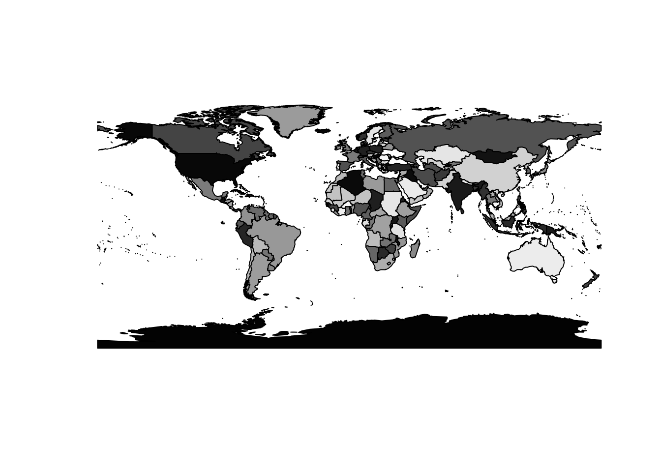
The R package maptools contains an in-built data set called wrld_simpl, which is a basic (and out of date) set of polygons describing the land masses of the world by country. This code loads the data set and plots it with a basic grey-scale scheme for individual countries.
class : SpatialPolygonsDataFrame
features : 246
extent : -180, 180, -90, 83.57027 (xmin, xmax, ymin, ymax)
variables : 11
# A tibble: 246 × 11
FIPS ISO2 ISO3 UN NAME AREA POP2005 REGION SUBREGION LON LAT
<fct> <fct> <fct> <int> <fct> <int> <dbl> <int> <int> <dbl> <dbl>
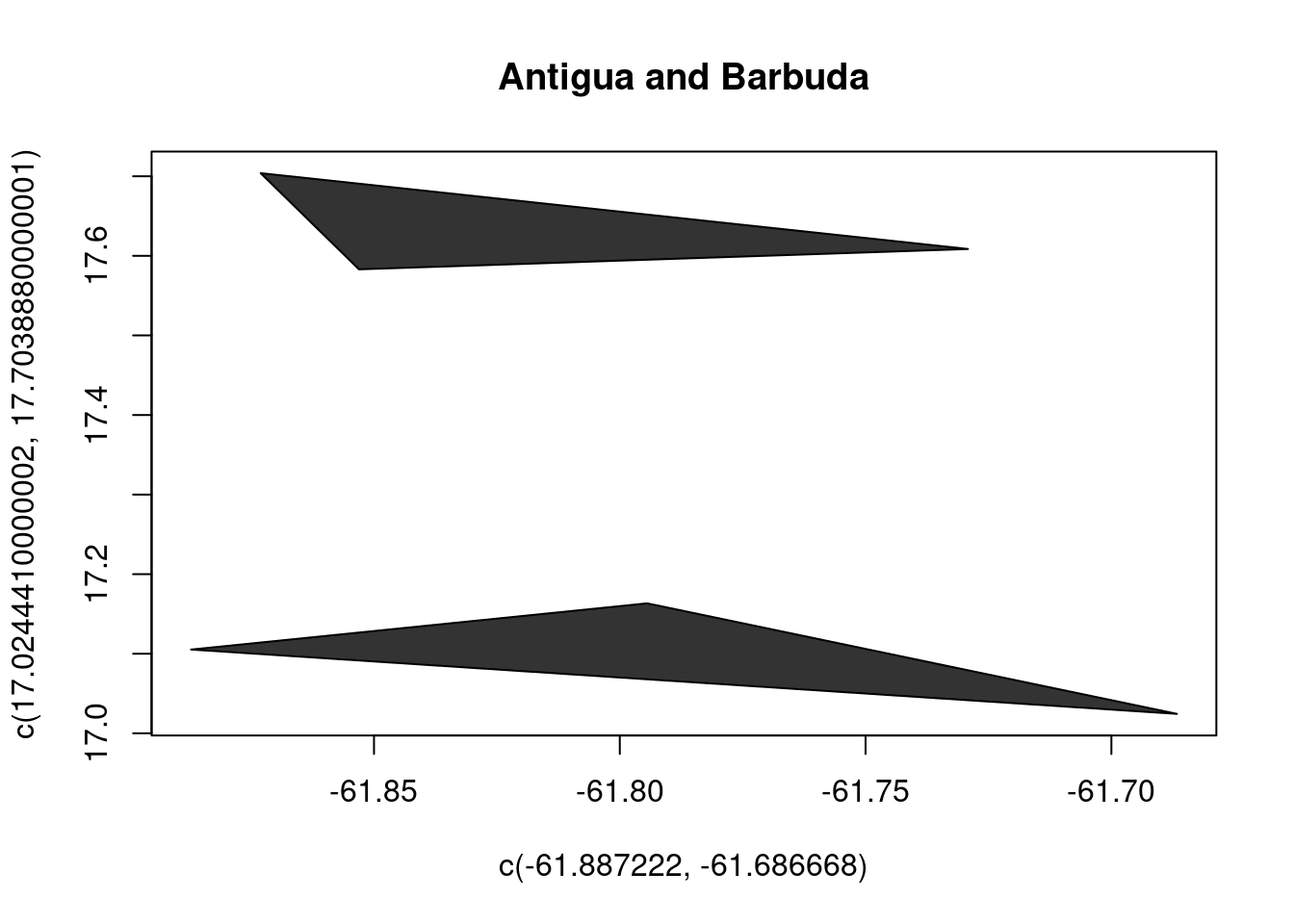
1 AC AG ATG 28 Antigu… 44 8.30e4 19 29 -61.8 17.1
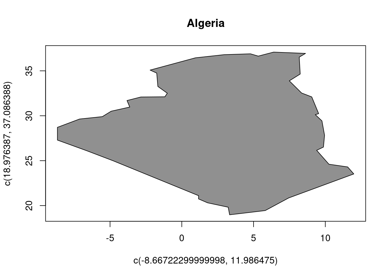
2 AG DZ DZA 12 Algeria 238174 3.29e7 2 15 2.63 28.2
3 AJ AZ AZE 31 Azerba… 8260 8.35e6 142 145 47.4 40.4
4 AL AL ALB 8 Albania 2740 3.15e6 150 39 20.1 41.1
5 AM AM ARM 51 Armenia 2820 3.02e6 142 145 44.6 40.5
6 AO AO AGO 24 Angola 124670 1.61e7 2 17 17.5 -12.3
7 AQ AS ASM 16 Americ… 20 6.41e4 9 61 -171. -14.3
8 AR AR ARG 32 Argent… 273669 3.87e7 19 5 -65.2 -35.4
9 AS AU AUS 36 Austra… 768230 2.03e7 9 53 136. -25.0
10 BA BH BHR 48 Bahrain 71 7.25e5 142 145 50.6 26.0
# … with 236 more rows
plot(wrld_simpl, col =grey(sample(seq(0, 1, length =nrow(wrld_simpl)))))
We also include a print statement to get a description of the data set, this is a SpatialPolygonsDataFrame which is basically a table of attributes with one row for each country, linked to a recursive data structure holding sets of arrays of coordinates for each individual piece of these complex polygons.
These structures are quite complicated, involving nested lists of matrices with X-Y coordinates. I can use class coercion from polygons, to lines, then to points as the most straightforward way of obtaining every XY coordinate by dropping the recursive hierarchy structure to get at every single vertex in one matrix.
(There are other methods to obtain all coordinates while retaining information about the country objects and their component “pieces”, but I’m ignoring that for now.)
We need to put these “X/Y” coordinates in 3D so I simply add another column filled with zeroes.
(Note for non-R users: in R expressions that don’t include assignment to an object with <- are generally just a side-effect, here the side effect of the head(allcoords) here is to print the top few rows of allcoords, just for illustration, there’s no other consequence of this code).
OpenGL in R
In R we have access to 3D visualizations in OpenGL via the rgl package, but the model for data representation is very different so I first plot the vertices of the wrld_simpl layer as points only.
library(rgl)plot3d(allcoords, xlab ="", ylab ="") ## smart enough to treat 3-columns as X,Y,Zrglwidget()
Plotting in the plane is one thing, but more striking is to convert the vertices from planar longitude-latitude to Cartesizan XYZ. Define an R function to take “longitude-latitude-height” and return spherical coordinates (we can leave WGS84 for another day).
llh2xyz <-function (lonlatheight, rad =6378137, exag =1) { cosLat =cos(lonlatheight[, 2] * pi/180) sinLat =sin(lonlatheight[, 2] * pi/180) cosLon =cos(lonlatheight[, 1] * pi/180) sinLon =sin(lonlatheight[, 1] * pi/180) rad <- (exag * lonlatheight[, 3] + rad) x = rad * cosLat * cosLon y = rad * cosLat * sinLon z = rad * sinLatcbind(x, y, z)}## deploy our custom function on the longitude-latitude valuesxyzcoords <-llh2xyz(allcoords)
Now we can visualize these XYZ coordinates in a more natural setting, and even add a blue sphere for visual effect.
This is still not very exciting, since our plot knows nothing about the connectivity between vertices.
Organization of polygons
The in-development R package gris provides a way to represent spatial objects as a set of relational tables. I’m leaving out the details because it’s not the point I want to make, but in short a gris object has tables “o” (objects), “b” (for branches), “bXv” (links between branches and vertices) and “v” the vertices.
If we ingest the wrld_simpl layer we get a list with several tables.
EDITOR NOTE (April 2022): see anglr function DEL0() for an updated way to create what gris was doing in 2015.
The objects, these are individual countries with several attributes including the NAME.
gobject$o
# A tibble: 246 × 12
FIPS ISO2 ISO3 UN NAME AREA POP2005 REGION SUBREGION LON LAT
<fct> <fct> <fct> <int> <fct> <int> <dbl> <int> <int> <dbl> <dbl>
1 AC AG ATG 28 Antigu… 44 8.30e4 19 29 -61.8 17.1
2 AG DZ DZA 12 Algeria 238174 3.29e7 2 15 2.63 28.2
3 AJ AZ AZE 31 Azerba… 8260 8.35e6 142 145 47.4 40.4
4 AL AL ALB 8 Albania 2740 3.15e6 150 39 20.1 41.1
5 AM AM ARM 51 Armenia 2820 3.02e6 142 145 44.6 40.5
6 AO AO AGO 24 Angola 124670 1.61e7 2 17 17.5 -12.3
7 AQ AS ASM 16 Americ… 20 6.41e4 9 61 -171. -14.3
8 AR AR ARG 32 Argent… 273669 3.87e7 19 5 -65.2 -35.4
9 AS AU AUS 36 Austra… 768230 2.03e7 9 53 136. -25.0
10 BA BH BHR 48 Bahrain 71 7.25e5 142 145 50.6 26.0
# … with 236 more rows, and 1 more variable: object_ <int>
The branches, these are individual simple, one-piece “ring polygons”. Every object may have one or more branches (branches may be an “island” or a “hole” but this is not currently recorded). Note how branch 1 and 2 (branch_) both belong to object 1, but branch 3 is the only piece of object 2.
This table is required so that we can normalize the vertices by removing any duplicates based on X/Y pairs. This is required for the triangulation engine used below, although not by the visualization strictly. (Note that we could also normalize branches for objects, since multiple objects might use the same branch - but again off-topic).
Finally, the vertices themselves. Here we only have X and Y, but these table structures can hold any number of attributes and of many types.
The normalization is only relevant for particular choices of vertices, so if we had X/Y/Z in use there might be a different version of “unique”. I think this is a key point for flexibility, some of these tasks must be done on-demand and some ahead of time.
Indices here are numeric, but there’s actually no reason that they couldn’t be character or other identifier. Under the hood the dplyr package is in use for doing straightforward (and fast!) table manipulations including joins between tables and filtering on values.
More 3D already!
Why go to all this effort just for a few polygons? The structure of the gris objects gives us much more flexibility, so I can for example store the XYZ Cartesian coordinates right on the same data set. I don’t need to recursively visit nested objects, it’s just a straightforward calculation and update - although we’re only making a simple point, this could be generalized a lot more for user code.
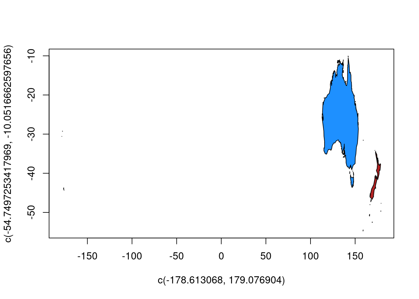
I now have XYZ coordinates for my data set, and so for example I will extract out a few nearby countries and plot them.
localarea <- gobject[gobject$o$NAME %in%c("Australia", "New Zealand"), ]## plot in traditional 2dplot(localarea, col =c("dodgerblue", "firebrick"))
The plot is a bit crazy since parts of NZ that are over the 180 meridian skews everything, and we could fix that easily by modifiying the vertex values for longitude, but it’s more sensible in 3D.
Finally, to get to the entire point of this discussion let’s triangulate the polygons and make a nice plot of the world.
The R package RTriangle wraps Jonathan Shewchuk’s Triangle library, allowing constrained Delaunay triangulations. To run this we need to make a Planar Straight Line Graph from the polygons, but this is fairly straightforward by tracing through paired vertices in the data set. The key parts of the PSLG are the vertices P and the segment indexes S defining paired vertices for each line segment. This is a “structural” index where the index values are bound to the actual size and shape of the vertices, as opposed to a more general but perhaps less efficient relational index.
The triangulation vertices (long-lat) can be converted to XYZ, and plotted.
xyz <-llh2xyz(cbind(tri$P, 0))open3d()
null
5
triangles3d(xyz[t(tri$T), ], col ="grey", specular ="black")aspect3d("iso"); bg3d("grey12")rglwidget()
These are very ugly polygons since there’s no internal vertices to carry the curvature of this sphere. This is the same problem we’d face if we tried to drape these polygons over topography: at some point we need internal structure.
Luckily Triangle can set a minimum triangle size. We set a constant minimum area, which means no individual triangle can be larger in area than so many “square degrees”. This gives a lot more internal structure so the polygons are more elegantly draped around the surface of the sphere. (There’s not really enough internal structure added with this minimum area, but I’ve kept it simpler to make the size of this document more manageable).
tri <- RTriangle::triangulate(pslgraph, a =9) ## a (area) is in degrees, same as our verticesxyz <-llh2xyz(cbind(tri$P, 0))open3d()
null
6
triangles3d(xyz[t(tri$T), ], col ="grey", specular ="black")bg3d("gray12")rglwidget()
We still can’t identify individual polygons as we smashed that information after putting the polygon boundary segments through the triangulator. With more careful work we could build a set of tables to store particular triangles between our vertices and objects, but to finish this story I just loop over each object adding them to the scene.
## loop over objectscols <-sample(grey(seq(0, 1, length =nrow(gobject$o))))open3d()
null
7
for (iobj inseq(nrow(gobject$o))) { pslgraph <- gris:::mkpslg(gobject[iobj, ]) tri <- RTriangle::triangulate(pslgraph, a =9) ## a is in units of degrees, same as our vertices xyz <-llh2xyz(cbind(tri$P, 0))triangles3d(xyz[t(tri$T), ], col = cols[iobj], specular ="black")}bg3d("gray12")rglwidget()