library(parallel)

worker_fun <- function(dates) {
  library(gdalraster)
  set_config_option("GDAL_DISABLE_READDIR_ON_OPEN", "EMPTY_DIR")
  era5 <- paste0('ZARR:"/vsicurl/https://storage.googleapis.com/',
                 'gcp-public-data-arco-era5/ar/',
                 '1959-2022-full_37-1h-0p25deg-chunk-1.zarr-v2"')
  ds <- new(GDALMultiDimRaster, era5)
  arr <- ds$openMDArray("/2m_temperature")
  dst <- sprintf("/vsimem/t2m_%d.tif", Sys.getpid())
  # PROJ reports "stere: Invalid latitude" for northern source points
  push_error_handler("quiet")
  on.exit({pop_error_handler(); arr$close(); ds$close()})
  vapply(dates, function(d) {
    t <- as.numeric(difftime(as.POSIXct(paste(d, "12:00:00"), tz = "UTC"),
                             as.POSIXct("1959-01-01", tz = "UTC"), units = "hours"))
    view <- arr$getView(sprintf("[%d,...]", t))
    r <- view$getUnscaled()$asClassicDataset(1, 0, NULL)
    warp(r, dst, t_srs = "EPSG:3031",
         cl_arg = c("-s_srs", "EPSG:4326", "-te", "-4000000", "-4000000",
                    "4000000", "4000000", "-tr", "25000", "25000",
                    "-r", "bilinear", "-wo", "SOURCE_EXTRA=2", "-overwrite"),
         quiet = TRUE)
    r$close(); view$close()
    out <- new(GDALRaster, dst)
    v <- out$read(1, 0, 0, 320, 320, 320, 320)
    out$close(); vsi_unlink(dst)
    v
  }, numeric(320 * 320))
}

worker_agg <- function(ym, worker_fun) {
  days <- unlist(lapply(ym, \(s) {
    d0 <- as.Date(paste0(s, "-01"))
    format(seq(d0, seq(d0, by = "month", length.out = 2)[2] - 1, by = "day"))
  }))
  X <- worker_fun(days)
  key <- substr(days, 1, 7)
  out <- vapply(ym, \(s) rowMeans(X[, key == s, drop = FALSE]), numeric(nrow(X)))
  list(ym = ym, n = as.integer(table(key)[ym]), mean = out)
}

ym <- format(seq(as.Date("1979-01-01"), as.Date("2021-12-01"), by = "month"), "%Y-%m")
cl <- makeCluster(32)
idx <- split(seq_along(ym), rep_len(seq_len(32), length(ym)))
res <- parLapply(cl, idx, \(i, f, w, y) f(y[i], w), worker_agg, worker_fun, ym)
stopCluster(cl)

monthly <- matrix(NA_real_, 320 * 320, length(ym), dimnames = list(NULL, ym))
nday <- integer(length(ym)); names(nday) <- ym
for (r in res) { monthly[, r$ym] <- r$mean; nday[r$ym] <- r$n }
saveRDS(list(ym = ym, ndays = nday, monthly_mean_K = monthly),
        "era5_t2m_3031_monthly_daily12utc.rds")
Note
This report was generated using AI under general human direction. At the time of generation, the contents have not been comprehensively reviewed by a human analyst.
This is a quick, rough-and-ready exploration of 2 m air temperature trends over Antarctica from the ERA5 reanalysis. The aim is a toy example of a real workload: read a remote 3-D Zarr array lazily with R powered by GDAL’s multidimensional API (the gdalraster package), warp each field to a polar stereographic grid, and compute per-pixel trends.
The data are the ARCO-ERA5 Zarr store on Google Cloud (hourly, 0.25 degrees, one global field per chunk). We sample one field per day at 12 UTC for 1979 to 2021, warp each to a 25 km EPSG:3031 grid, average to monthly means, and then to seasons. Trends are computed by ordinary least squares and checked with the Theil-Sen estimator, and the headline numbers are for Antarctic land (ice sheet and ice shelves) using ERA5’s own land-sea mask.
Method
Each field is one chunk of the array, so reading one hour costs one chunk fetch. For each date the pipeline is:
getView("[t,...]")selects one time step lazily (nothing is read).getUnscaled()$asClassicDataset(1, 0, NULL)turns the view into aGDALRasterwith x = longitude and y = latitude. This is also lazy.warp()reads only the block it needs and writes a 320 x 320 grid in EPSG:3031 (25 km, bilinear, extent of plus or minus 4000 km).
GDAL objects cannot be shared across R processes, so each of 32 PSOCK workers opens its own handle on the Zarr store and processes an interleaved share of the months. Each worker reduces its daily fields to monthly means before returning them, which keeps memory small.
The array’s time axis ends at the end of 2021, so the study period is 1979 to 2021. Time indices are hours since 1959-01-01 (this was assumed from the array’s layout, not read from its attributes).
The ice-sheet mask comes from the same store: the static /land_sea_mask array (a land fraction on the 0.25 degree grid, no time dimension) is warped to the same polar grid in the same way, and land is defined as warped fraction above 0.5. In ERA5 this treats ice shelves as land, so “land” here means ice sheet plus ice shelves plus islands inside the study disc.
Extraction code
These chunks are shown but not evaluated here: the temperature extraction took about 30 minutes for about 15,700 reads on 32 workers. The last chunk reduces that output to the small cache file this post is rendered from.
The land-sea mask is a single static field, so it is a one-off read (a few seconds):
library(gdalraster)
set_config_option("GDAL_DISABLE_READDIR_ON_OPEN", "EMPTY_DIR")
ds <- new(GDALMultiDimRaster, era5)   # `era5` is the ZARR:"/vsicurl/..." DSN above
arr <- ds$openMDArray("/land_sea_mask")  # dims: latitude, longitude
r <- arr$getUnscaled()$asClassicDataset(1, 0, NULL)
dst <- "/vsimem/lsm_3031.tif"
push_error_handler("quiet")
warp(r, dst, t_srs = "EPSG:3031",
     cl_arg = c("-s_srs", "EPSG:4326", "-te", "-4000000", "-4000000",
                "4000000", "4000000", "-tr", "25000", "25000",
                "-r", "bilinear", "-wo", "SOURCE_EXTRA=2", "-overwrite"),
     quiet = TRUE)
pop_error_handler()
r$close(); arr$close(); ds$close()
o <- new(GDALRaster, dst)
lsm <- o$read(1, 0, 0, 320, 320, 320, 320)
o$close(); vsi_unlink(dst)
The monthly means are then reduced to seasonal means, which is all the analysis needs. The days sampled in each month are used as weights, December is assigned to the following year’s DJF (so DJF 1979, which would lack December 1978, is dropped), and a season-year is kept only if all its months are present. Land pixels are stored at full seasonal resolution as integers in units of 0.01 K, a rounding that changes the land-mean trends by less than 1e-5 K/decade; the whole-disc mean of each season-year is stored at full precision. The cache is about 6 MB, against 220 MB for the monthly stack.
# `monthly`, `nday`, `ym` come from the extraction chunk; `lsm` from the mask chunk
xc <- -4e6 + 12500 + 25000 * (0:319)
grid <- expand.grid(x = xc, y = rev(xc))
inside <- sqrt(grid$x^2 + grid$y^2) <= 3.3e6
land_in <- (lsm > 0.5)[inside]

mo <- as.integer(substr(ym, 6, 7))
yr <- as.integer(substr(ym, 1, 4))
season_of <- c("DJF", "DJF", "MAM", "MAM", "MAM", "JJA",
               "JJA", "JJA", "SON", "SON", "SON", "DJF")[mo]
season_year <- ifelse(mo == 12, yr + 1, yr)

# Weighted mean over the months of each complete season-year
aggregate_seasons <- function(sel, key, n_months) {
  years <- sort(unique(key[sel]))
  Y <- lapply(years, \(y) {
    k <- which(sel & key == y)
    if (length(k) != n_months) return(NULL)
    as.vector(monthly[inside, k, drop = FALSE] %*% nday[k] / sum(nday[k]))
  })
  keep <- !vapply(Y, is.null, logical(1))
  list(years = years[keep], Y = do.call(cbind, Y[keep]))
}

seasons <- c("DJF", "MAM", "JJA", "SON")
sm <- c(
  setNames(lapply(seasons, \(s) aggregate_seasons(season_of == s, season_year, 3)), seasons),
  list(Annual = aggregate_seasons(rep(TRUE, length(ym)), yr, 12))
)

small <- list(
  meta = list(first_month = ym[1], last_month = ym[length(ym)], n_months = length(ym),
              total_days = sum(nday), missing_in_disc = sum(is.na(monthly[inside, ])),
              disc_pixels = sum(inside), land_pixels = sum(land_in), pixel_km2 = 625),
  land_fraction = lsm,
  seasons = lapply(sm, \(z) list(
    years = z$years,
    Y_cK = `storage.mode<-`(round(z$Y[land_in, , drop = FALSE] * 100), "integer"),
    disc_mean_K = colMeans(z$Y)))
)
saveRDS(small, "era5_t2m_3031_seasonal_land.rds", compress = "xz")
Load and check the cache
library(ggplot2)small <- readRDS("era5_t2m_3031_seasonal_land.rds")
meta <- small$meta
# pixel centres of the 320 x 320 grid; rows are read top-down
xc <- -4e6 + 12500 + 25000 * (0:319)
grid <- expand.grid(x = xc, y = rev(xc))
# disc of radius 3300 km, roughly south of 60S (includes ocean and sea ice)
inside <- sqrt(grid$x^2 + grid$y^2) <= 3.3e6
# land = ice sheet, ice shelves and islands (ERA5 land fraction above 0.5)
land <- small$land_fraction > 0.5
grid <- grid[inside, ]
land_in <- land[inside]
# seasonal means (K) at land pixels, and the whole-disc mean per season-year
sm <- lapply(small$seasons, \(z) list(years = z$years,
Y = z$Y_cK / 100,
disc_mean = z$disc_mean_K))stopifnot(sum(land_in) == meta$land_pixels, sum(inside) == meta$disc_pixels)
c(land_pixels = nrow(sm$DJF$Y),
vapply(sm, \(z) length(z$years), integer(1)))land_pixels DJF MAM JJA SON Annual
21857 42 43 43 43 43 The cache was built from 516 monthly means (1979-01 to 2021-12) of 15,706 daily fields, with 0 missing values inside the analysis disc. Of the 54,756 pixels in the disc, 21,857 are land, which is about 13.7 million km^2 at 625 km^2 per pixel (a sanity check against Antarctica’s area including ice shelves, roughly 14 million km^2).
ggplot(cbind(grid, land = land_in), aes(x, y, fill = land)) +
  geom_raster() +
  coord_equal() +
  labs(title = "ERA5 land mask on the 25 km polar grid", x = NULL, y = NULL)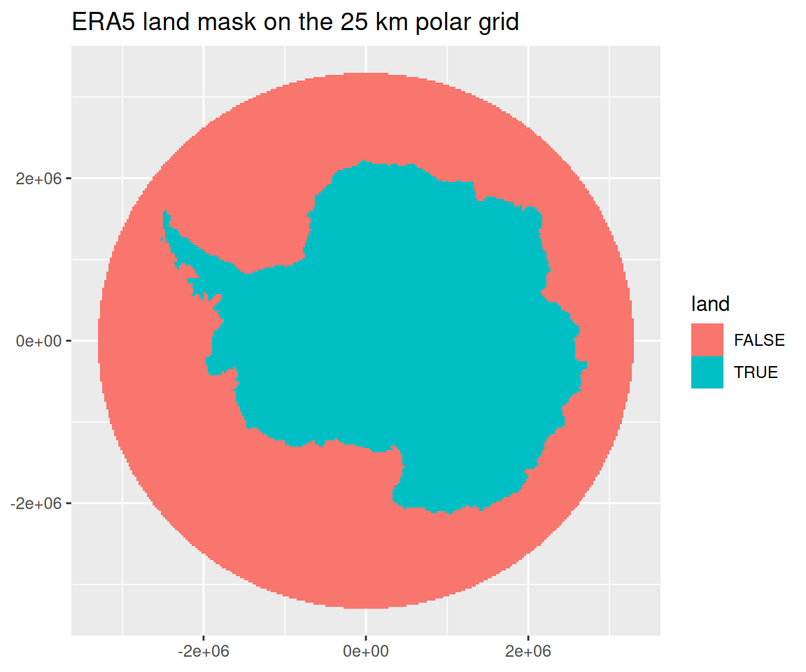
Seasonal means and trends
The seasons are DJF, MAM, JJA and SON, plus the annual mean, formed from monthly means as described in the extraction section (December belongs to the following year’s DJF, and only complete season-years are used).
The per-pixel trend is an ordinary least squares slope of seasonal mean against year, in K per decade, with its t statistic. The Theil-Sen slope is the median of all pairwise slopes between years, which is robust to individual outlying years. Everything from here on uses land pixels only.
trend <- function(Y, years) {
  x <- (years - mean(years)) / 10
  b <- as.vector(Y %*% x) / sum(x^2)
  res <- Y - rowMeans(Y) - outer(b, x)
  se <- sqrt(rowSums(res^2) / (length(x) - 2) / sum(x^2))
  data.frame(slope = b, t = b / se)
}

# Theil-Sen per row of Y (pixels x years), in units per decade
theil_sen_rows <- function(Y, years) {
  pr <- combn(length(years), 2)
  dx <- (years[pr[2, ]] - years[pr[1, ]]) / 10
  D <- (Y[, pr[2, ], drop = FALSE] - Y[, pr[1, ], drop = FALSE]) |>
    sweep(2, dx, "/")
  apply(D, 1, median)
}

# Theil-Sen for a single series, per decade
theil_sen <- function(y, years) {
  pr <- combn(length(years), 2)
  median((y[pr[2, ]] - y[pr[1, ]]) / ((years[pr[2, ]] - years[pr[1, ]]) / 10))
}

trends <- do.call(rbind, lapply(names(sm), \(s) {
  tr <- trend(sm[[s]]$Y, sm[[s]]$years)
  tr$theil_sen <- theil_sen_rows(sm[[s]]$Y, sm[[s]]$years)
  cbind(grid[land_in, ], tr, season = factor(s, names(sm)))
}))
trends$slope_sig <- ifelse(abs(trends$t) > 2, trends$slope, NA)
Trend maps over land
The maps show Antarctic land only, with the OLS slope. Pixels with |t| < 2 are shown in grey. With about 21,857 strongly spatially correlated pixels per map, and years treated as independent, this is a descriptive filter and not a test with controlled error.
ggplot(trends, aes(x, y, fill = slope_sig)) +
  geom_raster() +
  scale_fill_gradient2(name = "K/decade", low = "blue", high = "red",
                       na.value = "grey85") +
  facet_wrap(~season) +
  coord_equal() +
  labs(title = "ERA5 2 m temperature trend over land, 1979-2021 (daily 12 UTC)",
       subtitle = "OLS slope; grey: |t| < 2", x = NULL, y = NULL)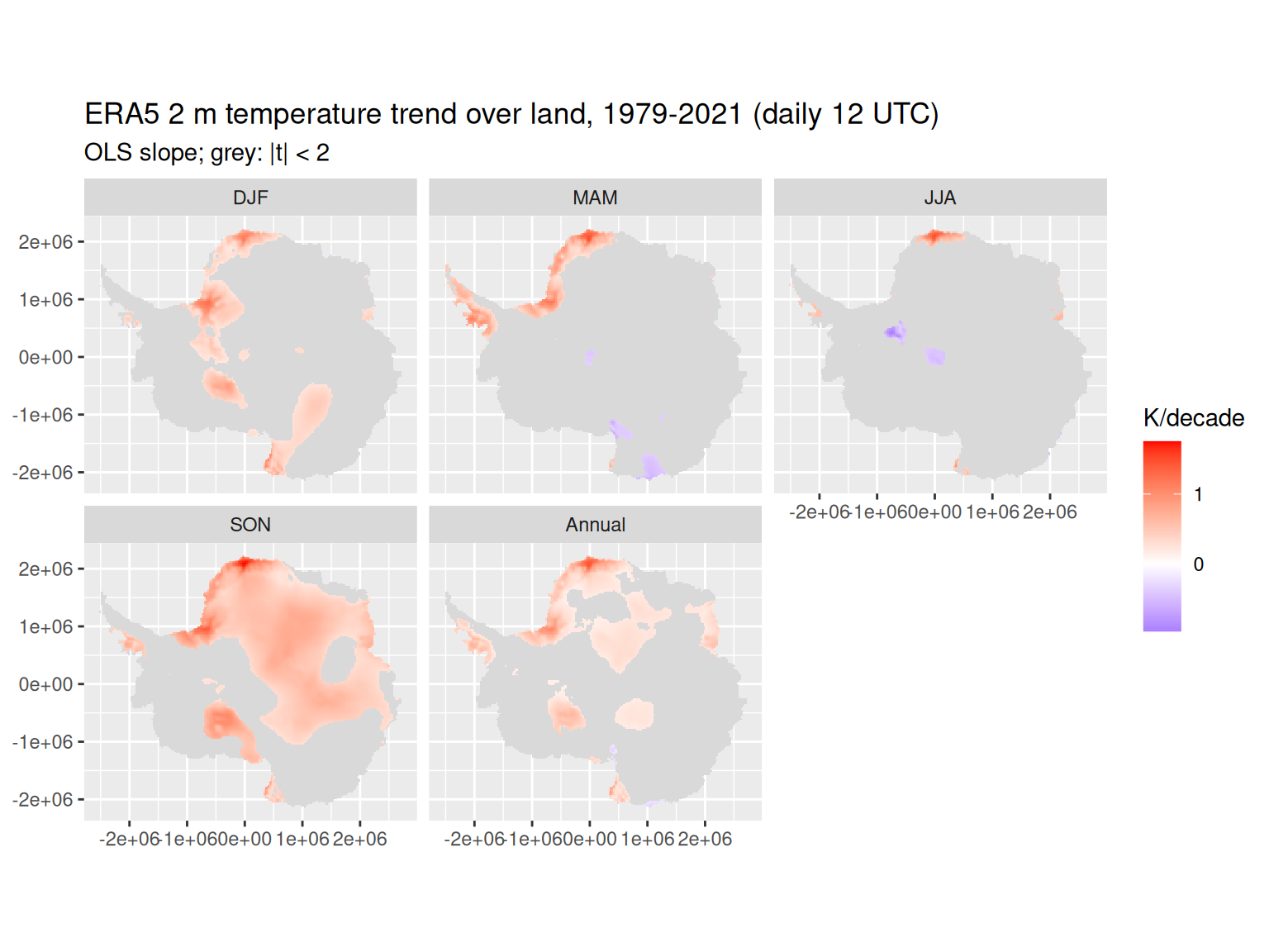
land_tr <- trends
frac_sig <- tapply(abs(land_tr$t) > 2, land_tr$season, mean)
round(100 * frac_sig, 1)
DJF MAM JJA SON Annual
17.2 9.2 3.1 50.6 24.5 The share of land pixels with |t| > 2 ranges from 3% (JJA) to 51% (SON). About 5% would be expected by chance alone under independence (JJA is below that level). The spatial patches are what carry the information, and they should not be read pixel by pixel.
Theil-Sen check, per pixel
If a few anomalous years drove the OLS slopes, the Theil-Sen slopes would differ from them. The plot compares the two on every land pixel.
ggplot(land_tr, aes(slope, theil_sen)) +
  geom_point(size = 0.2, alpha = 0.2) +
  geom_abline(colour = "red") +
  facet_wrap(~season) +
  coord_equal() +
  labs(x = "OLS slope (K/decade)", y = "Theil-Sen slope (K/decade)")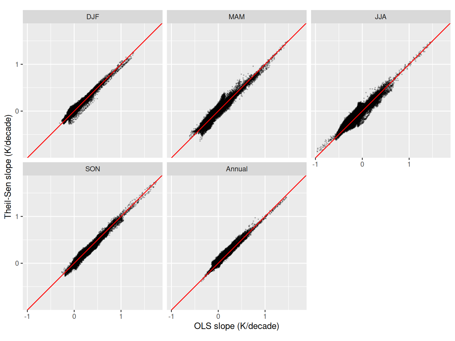
agree <- do.call(rbind, lapply(split(land_tr, land_tr$season), \(z) {
  data.frame(correlation = cor(z$slope, z$theil_sen),
             median_abs_diff = median(abs(z$slope - z$theil_sen)),
             median_ols = median(z$slope), median_theil_sen = median(z$theil_sen))
}))
knitr::kable(agree, digits = 3,
             col.names = c("Correlation", "Median |OLS - TS|",
"Median OLS", "Median TS"))| Correlation | Median |OLS - TS| | Median OLS | Median TS | |
|---|---|---|---|---|
| DJF | 0.983 | 0.021 | 0.096 | 0.100 |
| MAM | 0.967 | 0.040 | 0.009 | 0.021 |
| JJA | 0.946 | 0.046 | -0.011 | 0.018 |
| SON | 0.987 | 0.030 | 0.345 | 0.320 |
| Annual | 0.971 | 0.024 | 0.103 | 0.112 |
Across land pixels the two estimators are highly correlated (correlation of 0.95 or more in every season), and the median absolute difference between them is at most 0.05 K/decade. So the OLS maps are not being driven by a handful of extreme years.
Continental mean series
The headline series is the unweighted mean over land pixels. For comparison, the mean over the whole disc (which includes ocean and sea ice) is also shown.
series <- do.call(rbind, lapply(names(sm), \(s) {
  rbind(
    data.frame(year = sm[[s]]$years, season = factor(s, names(sm)), domain = "Land",
               t2m = colMeans(sm[[s]]$Y) - 273.15),
    data.frame(year = sm[[s]]$years, season = factor(s, names(sm)), domain = "Whole disc",
               t2m = sm[[s]]$disc_mean - 273.15)
  )
}))

ggplot(subset(series, domain == "Land"), aes(year, t2m)) +
  geom_line() +
  geom_smooth(method = "lm", se = FALSE) +
  facet_wrap(~season, scales = "free_y") +
  labs(title = "Land mean 2 m temperature", y = "2 m temperature (degC)", x = NULL)
`geom_smooth()` using formula = 'y ~ x'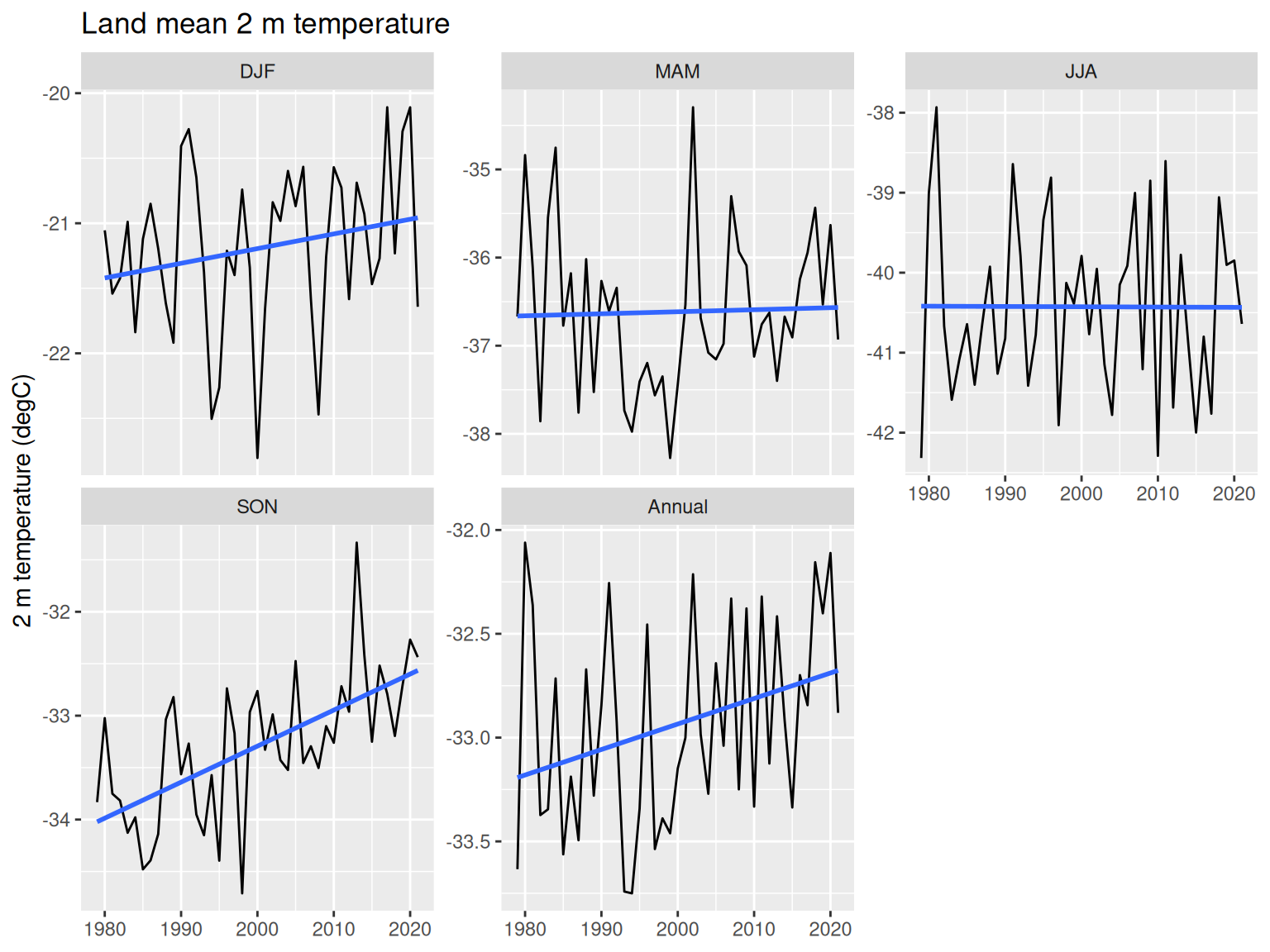
fit <- \(z) {
  m <- lm(t2m ~ I(year / 10), z)
  c(ols = unname(coef(m)[2]), se = unname(coef(summary(m))[2, 2]),
    theil_sen = theil_sen(z$t2m, z$year))
}
tab_of <- \(d) t(sapply(split(d, d$season), fit))
land_all <- tab_of(subset(series, domain == "Land"))
land_80 <- tab_of(subset(series, domain == "Land" & year >= 1980))
disc_all <- tab_of(subset(series, domain == "Whole disc"))

tab <- data.frame(
  season = rownames(land_all),
  land_ols = land_all[, "ols"], land_se = land_all[, "se"],
  land_ts = land_all[, "theil_sen"],
  land_ols_1980 = land_80[, "ols"], land_ts_1980 = land_80[, "theil_sen"],
  disc_ols = disc_all[, "ols"], disc_ts = disc_all[, "theil_sen"],
  row.names = rownames(land_all)
)
knitr::kable(tab, digits = 3, row.names = FALSE,
             col.names = c("Season", "Land OLS", "SE", "Land Theil-Sen",
                           "Land OLS from 1980", "Land TS from 1980",
"Disc OLS", "Disc TS"))| Season | Land OLS | SE | Land Theil-Sen | Land OLS from 1980 | Land TS from 1980 | Disc OLS | Disc TS |
|---|---|---|---|---|---|---|---|
| DJF | 0.113 | 0.080 | 0.111 | 0.113 | 0.111 | 0.014 | -0.001 |
| MAM | 0.023 | 0.112 | 0.092 | 0.023 | 0.110 | -0.038 | -0.022 |
| JJA | -0.004 | 0.137 | 0.024 | -0.070 | -0.022 | -0.054 | -0.066 |
| SON | 0.347 | 0.066 | 0.343 | 0.353 | 0.346 | 0.161 | 0.157 |
| Annual | 0.123 | 0.058 | 0.144 | 0.107 | 0.133 | 0.023 | 0.030 |
All trends are in K/decade. The land mean trend is largest in SON, at 0.35 (OLS, standard error 0.07, about 5.2 standard errors from zero) and 0.34 by Theil-Sen. The annual land trend is 0.12 (about 2.1 standard errors, borderline given the naive standard errors), DJF is 0.11 (1.4 standard errors), and MAM and JJA are indistinguishable from zero. The land-mean Theil-Sen and OLS slopes differ by at most 0.07 K/decade across seasons, well inside the OLS standard errors, so the series-level conclusions do not depend on the estimator.
The land mean trends are larger than the whole-disc trends in DJF, SON and the annual mean (for example SON 0.16 over the disc against 0.35 over land). This is consistent with weaker trends over the ocean and sea-ice part of the disc diluting the disc mean, although the ocean-only mean was not computed separately here. Dropping 1979 changes the JJA land OLS estimate from -0.00 to -0.07 K/decade, which is small relative to its standard error of 0.14.
Caveats
- These are reanalysis trends. Antarctic 2 m temperature in ERA5 depends on the model and on the observations assimilated, which are sparse and changed over time (especially before 1979, which is why the period starts there).
- Sampling is one field per day at 12 UTC, not full daily means, so the diurnal cycle is not averaged out. A fixed hour is unlikely to bias trends much but adds noise.
- The land mask is ERA5’s own land fraction (above 0.5) warped bilinearly to 25 km. It treats ice shelves as land and has coarse (0.25 degree) coastlines, so coastal pixels mix land and ocean influence. It is not a survey-grade ice-sheet outline.
- Pixels are weighted equally on the 25 km EPSG:3031 grid, which is only approximately equal-area (a scale error of about 1.5% at 60 degrees S).
- The t statistics assume independent years, ignore autocorrelation and spatial correlation, and are not corrected for the number of pixels. Treat maps as descriptive. Theil-Sen is used here as a robustness check on the slope, not to provide a significance test.
- The time index (hours since 1959-01-01) was assumed from the array layout, and the 2022 index is not available in the array, so the series stops at 2021.
Reproducibility
The extraction chunks need a GDAL build with the multidimensional API and Zarr driver, the development build of gdalraster with GDALMultiDimRaster views, and network access to the public Google Cloud bucket. The rest of the document only needs the roughly 6 MB cache file era5_t2m_3031_seasonal_land.rds next to this file.
sessionInfo()R version 4.6.1 (2026-06-24)
Platform: x86_64-pc-linux-gnu
Running under: Ubuntu 24.04.5 LTS
Matrix products: default
BLAS: /usr/lib/x86_64-linux-gnu/openblas-pthread/libblas.so.3
LAPACK: /usr/lib/x86_64-linux-gnu/openblas-pthread/libopenblasp-r0.3.26.so; LAPACK version 3.12.0
locale:
[1] LC_CTYPE=en_AU.UTF-8 LC_NUMERIC=C
[3] LC_TIME=en_AU.UTF-8 LC_COLLATE=en_AU.UTF-8
[5] LC_MONETARY=en_AU.UTF-8 LC_MESSAGES=en_AU.UTF-8
[7] LC_PAPER=en_AU.UTF-8 LC_NAME=C
[9] LC_ADDRESS=C LC_TELEPHONE=C
[11] LC_MEASUREMENT=en_AU.UTF-8 LC_IDENTIFICATION=C
time zone: Etc/UTC
tzcode source: system (glibc)
attached base packages:
[1] stats graphics grDevices utils datasets methods base
other attached packages:
[1] ggplot2_4.0.3
loaded via a namespace (and not attached):
[1] Matrix_1.7-6 gtable_0.3.6 jsonlite_2.0.0 dplyr_1.2.1
[5] compiler_4.6.1 tidyselect_1.2.1 parallel_4.6.1 dichromat_2.0-1
[9] splines_4.6.1 scales_1.4.0 yaml_2.3.12 fastmap_1.2.0
[13] lattice_0.23-1 R6_2.6.1 labeling_0.4.3 generics_0.1.4
[17] knitr_1.52 htmlwidgets_1.6.4 tibble_3.3.1 pillar_1.11.1
[21] RColorBrewer_1.1-3 rlang_1.3.0 xfun_0.60 S7_0.2.2
[25] otel_0.2.0 cli_3.6.6 withr_3.0.3 magrittr_2.0.5
[29] mgcv_1.9-4 digest_0.6.39 grid_4.6.1 rstudioapi_0.19.0
[33] rappdirs_0.3.4 lifecycle_1.0.5 nlme_3.1-171 vctrs_0.7.3
[37] evaluate_1.0.5 glue_1.8.1 farver_2.1.2 rmarkdown_2.32
[41] tools_4.6.1 pkgconfig_2.0.3 htmltools_0.5.9